Chapter 3 Components of a Time Series
A given time series can have four possible components:
Trend: denoted by \(B_t\) captures the long run behavior of the time series of interest.
Season: denoted by \(S_t\) are periodic fluctuations over seasons. The period of the season is fixed and known. For example, rise in non-durable sales during Christmas.
Cycle: denoted by \(C_t\) are non-periodic fluctuations in that they occur regularly but over periods that are not fixed in duration.
Irregular: denoted by \(\epsilon_t\) are random fluctuations, typically modeled as a white noise process.
3.1 Decomposing a time series
We can decompose any given time series into its components. There are two ways to accomplish this:
Additive Decomposition: Here it is assumed that all four components are added to obtain the underlying time series: \[\begin{equation} y_t= B_t+S_t+C_t +\epsilon_t \end{equation}\]
Multiplicative Decomposition: Here it is assumed that all four components are multiplied to obtain the underlying time series: \[\begin{equation} y_t= B_t \times S_t \times C_t \times \epsilon_t \end{equation}\]
Note that using properties of logarithms, multiplicative decomposition is the same as additive decomposition in log terms: \[\begin{equation} log(y_t)= log(B_t) + log(S_t) + log(C_t) + log(\epsilon_t) \end{equation}\]
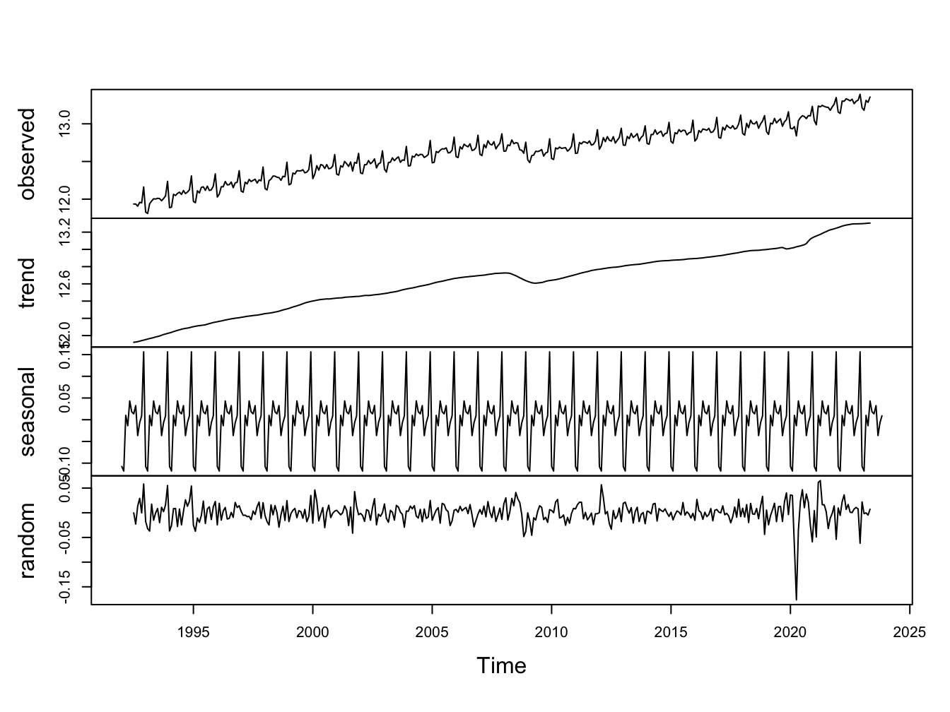
Most statistical software can implement these decomposition using data on a time series variable as input. Typically they combine cyclical component with irregular component and provide a three-way decomposition. In Figure 3.1 I use R to decompose real GDP for the US into its components.

Figure 3.1: Additive Decomposition of Retail Sales
3.2 Uses of Decomposition of a time series
The usefulness of decomposing a time series depends on our objective.
It may be of interest to study each component separately or to simply improve our understanding of the temporal dynamics of a time series of interest. Decomposing it into different components is the first step towards achieving that goal.
We can also use the decomposition to filter out components that we are not interested in studying. If for example we are only interested in modeling the cyclical component of the time series, then we can assume some kind decomposition, additive or multiplicative, and filter out the trend and seasonal component. For example, assuming additive decomposition, the filtered time series is given by: \[\begin{equation} Filtered \ y_t= y_t-B_t-S_t \end{equation}\]
We can then proceed to model the cyclical component using the filtered data.