Chapter 1 Introduction to Forecasting

1.1 Time Series

A time series is a specific kind of data where observations of a variable are recorded over time. For example, the data for the U.S. GDP for the last 30 years is a time series data.

Such data shows how a variable is changing over time. Depending on the variable of interest we can have data measured at different frequencies. Some commonly used frequencies are intra-day, daily, weekly, monthly, quarterly, semi-annual and annual. Figure 1.1 below plots data for quarterly and monthly frequency.

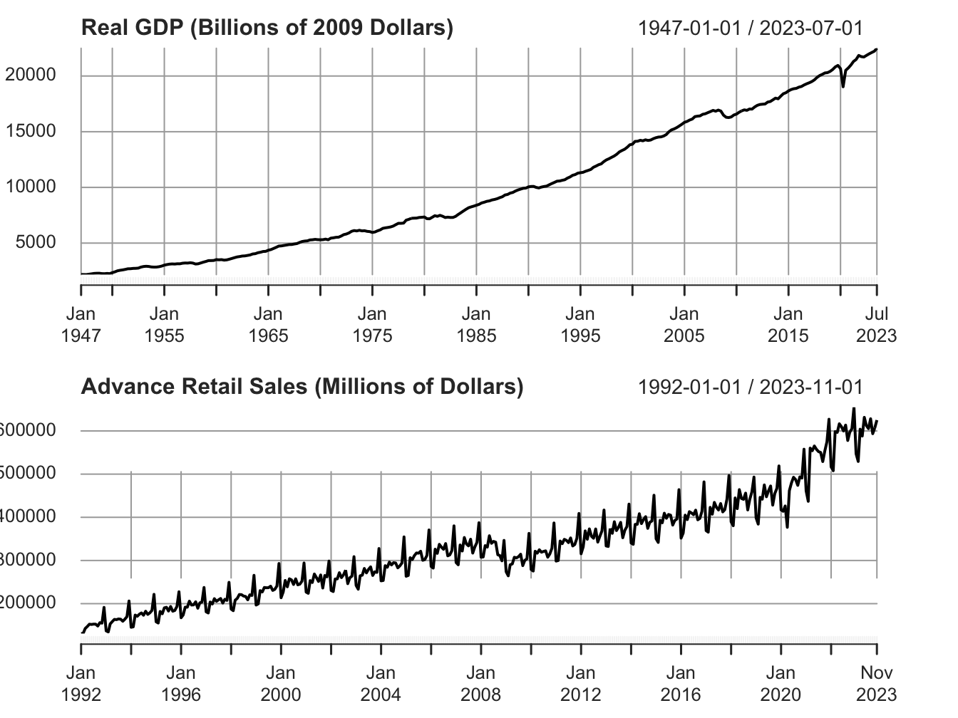
Figure 1.1: Time Series at quarterly and monthly frequency

The first panel shows data for the real gross domestic product (GDP) for the US in billions of 2012 dollars, measured at a quarterly frequency. The second panel shows data for the advance retail sales (millions of dollars), measured at monthly frequency.

Formally, we denote a time series variable by \(y_t\), where \(t=0,1,2,..,T\) is the observation index. For example, at \(t=10\) we get the tenth observation of this time series, \(y_{10}\).

1.2 Serial Correlation

Serial correlation (or auto correlation) refers to the tendency of observations of a time series being correlated over time. It is a measure of the temporal dynamics of a time series and addresses the following question: what is the effect of past realizations of a time series on the current period value? Formally,

\[\begin{equation} \rho(s)=Cor(y_t, y_{t-s}) =\frac{ Cov(y_t,y_{t-s})}{\sqrt{\sigma^2_{y_t} \times \sigma^2_{y_{t-s}}}} \tag{1.1} \end{equation}\]

where \(Cov(y_t,y_{t-s})= E(y_t-\mu_{y_t})(y_{t-s}-\mu_{y_{t-s}})\) and \(\sigma^2_{y_t}=E(y_t-\mu_{y_t})^2\)

Here, \(\rho(s)\) is the serial correlation of order \(s\). For example, \(s=1\) implies first order serial correlation between \(y_t\) and \(y_{t-1}\), \(s=2\) implies second order serial correlation between \(y_t\) and \(y_{t-2}\), and so on.

Note that often we use historical data to forecast. If there is no serial correlation, then past can offer no guidance for the present and future. In that sense, presence of serial correlation of some order is the first condition for being able to forecast a time series using its historical realizations.

Now, we can either have positive or negative serial correlation in data. Figure ?? plots two time series with positive and negative serial correlation, respectively.

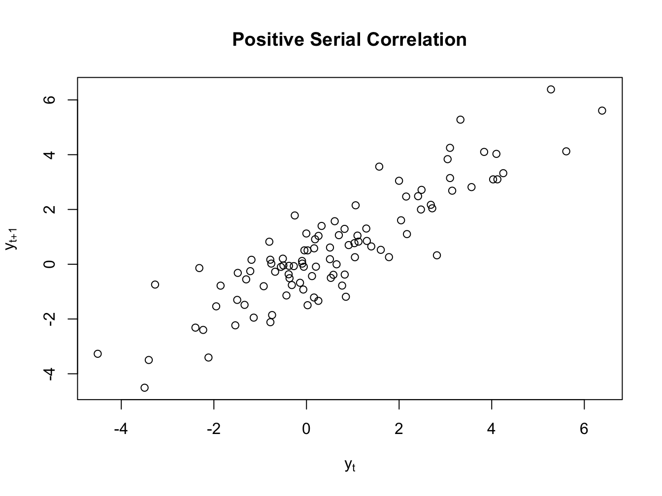
Figure 1.2: Serial Correlation

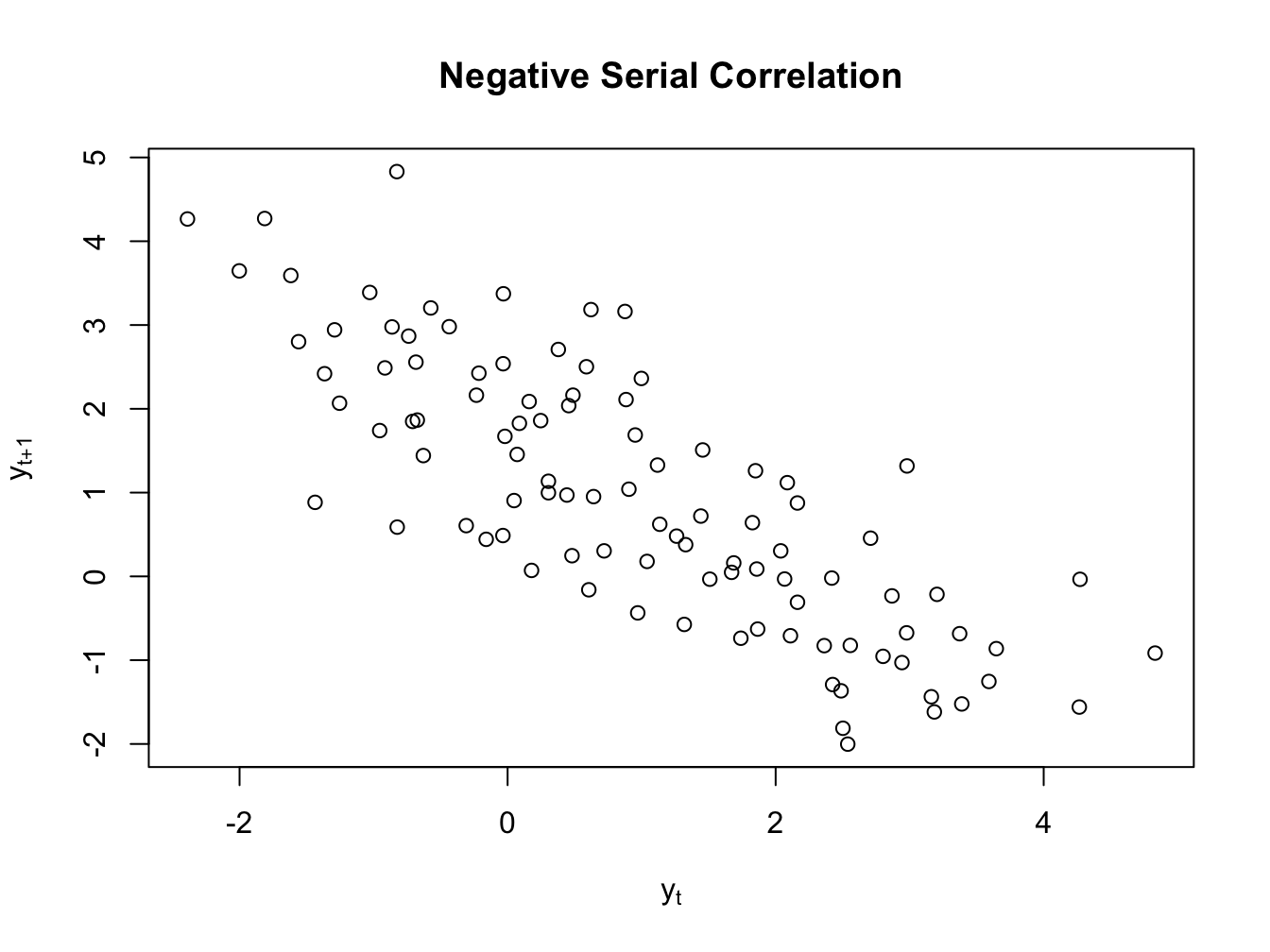
Figure 1.3: Serial Correlation

1.3 Testing for Serial Correlion

We can use a Lagrange-Multiplier (LM) test for detecting serial correlation. This test is also known as Breuch-Godfrey test. I will use the linear regression model to explain this test. Consider the following regression model: \[\begin{equation} y_t=\beta_0 + \beta_1 X_{1t}+\epsilon_t \end{equation}\]

Consider the following model for serial correlation of order p for the error term: \[\begin{equation} \epsilon_t=\rho_1 \epsilon_{t-1}+\rho_2 \epsilon_{t-2}+...+ \rho_p \epsilon_{t-p}+\nu_t \tag{1.2} \end{equation}\]

Then we are interested in the following test:

\[H_0=\rho_1=\rho_2=...=\rho_p=0 \] \[H_A = Not \ H_0 \]

To implement this test, we estimate the BG regression model given by: \[\begin{equation} e_t=\alpha_0 + \alpha_1 X_{1t}+ \rho_1 e_{t-1}+\rho_2 e_{t-2}+...+ \rho_p e_{t-p}+\nu_t \tag{1.3} \end{equation}\]

where we replace the error term with the OLS residuals (denoted by \(e\)). The LM test statistic is given by:

\[ LM = N\times R^2_{BG} \sim \chi^2_p \]

If the test statistic value is greater than the critical value then we reject the null hypothesis.

1.4 White Noise Process

Definition 1.1 (White Noise)

A time series is a white noise process if it has zero mean, constant and finite variance, and is serially uncorrelated. Formally, \(y_t\) is a white noise process if:

1. \(E(y_t)=0\)
2. \(Var(y_t)=\sigma^2_y\)
3. \(Cov(y_t,y_{t-s})= 0 \forall s\neq t\)

We can compress the above definition as: \(y_t\sim WN(0,\sigma^2_y)\). Often we assume that the unexplained part of a time series follows a white noise process. Formally,

\[\begin{equation} Time \ Series \ = \ Explained \ + \ White \ Noise \end{equation}\]

By definition we cannot forecast a white noise process. An important diagnostics of model adequacy is to test whether the estimated residuals are white noise (more on this later).

1.5 Important Elements of Forecasting

Definition 1.2 (Forecast)

A forecast is an informed guess about the unknown future value of a time series of interest. For example, what is the stock price of Facebook next Monday?

There are three possible types of forecasts:

1. Density Forecast: we forecast the entire probability distribution of the possible future value of the time series of interest. Hence,

\[\begin{equation} F(a)=P[y_{t+1}\leq a] \end{equation}\]

give us the probability that the 1-period ahead future value of \(y_{t+1}\) will be less than or equal to \(a\). For example, the future real GDP growth could be normally distributed with a mean of 1.3% and a standard deviation of 1.83%. Figure 1.4 below plots the density forecast for real GDP growth.

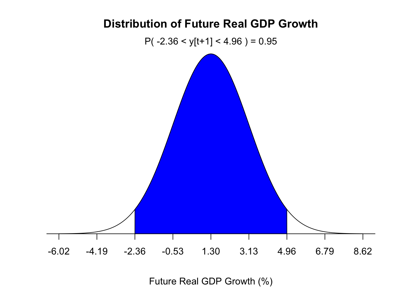
Figure 1.4: Density Forecast for Future Real GDP Growth

2. Point Forecast: our forecast at each horizon is a single number. Often we use the expected value or mean as the point forecast. For example, the point forecast for the 1-period ahead real GDP growth can be the mean of the probability distribution of the future real GDP growth: \[\begin{equation} f_{t,1}=1.3% \end{equation}\]

3. Interval Forecast: our forecast at each horizon is a range which is obtained by adding margin of errors to the point forecast. With some probability we expect our future value to fall withing this range. For example, the 95% interval forecast for the next period real GDP growth is (-2.36%,4.96%). Hence, with 95% confidence we expect next period GDP to fall between -2.36% and 4.96%.

Definition 1.3 (Forecast Horizon)

Forecast Horizon is the number of periods into the future for which we forecast a time series. We will denote it by \(h\). Hence, for \(h=1\), we are looking at 1-period ahead forecast, for \(h=2\) we are looking at 2-period ahead forecast and so on.

Formally, for a given time series \(y_t\), the h-period ahead unknown value is denoted by \(y_{t+h}\). The forecast of this value is denoted \(f_{t,h}\).

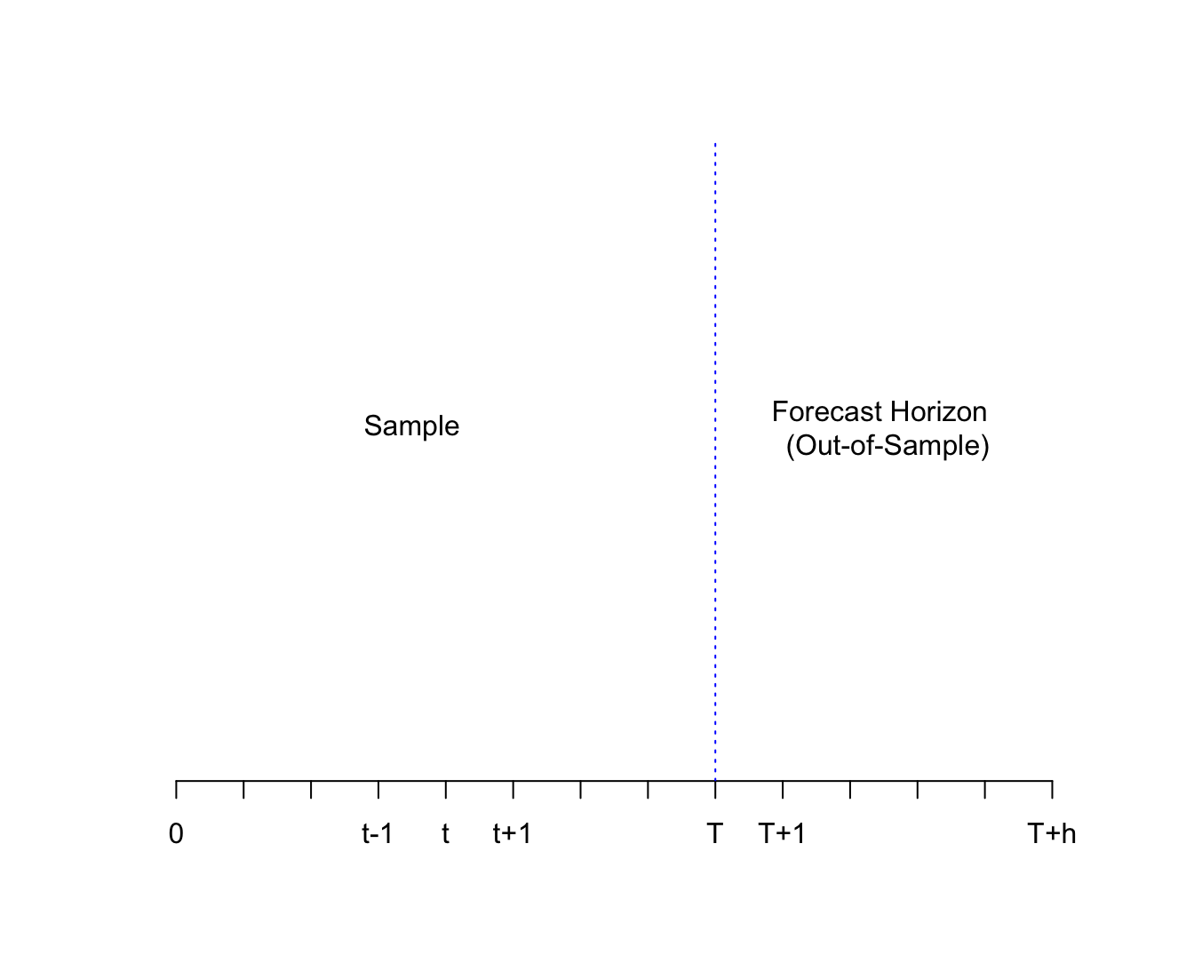
Figure 1.5: Forecast Horizon

Definition 1.4 (Forecast Error)

A forecast error is the difference between the realization of the future value and the previously made forecast. Formally, the \(h\)-period ahead forecast error is given by:

\[\begin{equation} e_{t,h}=y_{t+h}-f_{t,h} \end{equation}\]

Hence, for every horizon, we will have a forecast and a corresponding forecast error. These errors can be negative (indicating over prediction) or positive (indicating under prediction).

Forecasts are based on information available at the time of making the forecast. Information Set contains all the relevant information about the time series we would like to forecast. We denote the set of information available at time \(T\) by \(\Omega_T\). There are two types of information sets:

1. Univariate Information set: Only includes historical data on the time series of interest: \[\begin{equation} \Omega_T=\{y_T, y_{T-1}, y_{T-2}, ...., y_1\} \end{equation}\]

2. Multivariate Information set: Includes historical data on the time series of interest as well as any other variable(s) of interest. For example, suppose we have one more variable \(x\) that is relevant for forecasting \(y\). Then: \[\begin{equation} \Omega_T=\{y_T, x_T, y_{T-1}, x_{T-1}, y_{T-2},x_{T-2}. ...., y_1, x_1\} \end{equation}\]

1.6 Loss Function and Optimal Forecast

Think of a forecast as a solution to an optimization problem. When forecasts are wrong, the person making the forecast will suffer some loss. This loss will be a function of the magnitude as well as the sign of the forecast error. Hence, we can think of an optimal forecast as a solution to a minimization problem where the forecaster is minimizing the loss from the forecast error.

Definition 1.5 (Loss Function)

A loss function is a mapping between forecast errors and their associated losses. Formally, we denote the h-period ahead loss function by \(L(e_{t,h})\). For a function to be used as a loss function, three properties must be satisfied:

1. \(L(0)=0\)
2. \(\frac{dL}{de}>0\)
3. \(L(e)\) is a continuous function.

Two types of loss functions are:

• Symmetric Loss Function: both positive and negative forecast errors lead to same loss. See Figure 1.6. A commonly used loss function is quadratic loss function given by:

\[\begin{equation} L(e_{t,h})=e_{t,h}^2 = (y_{t+h}-f{t,h})^2 \end{equation}\]

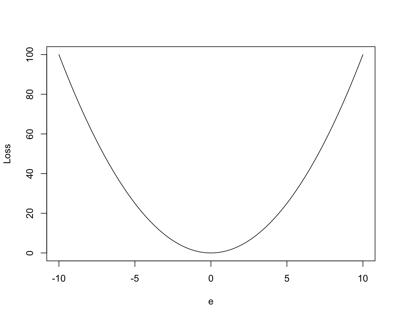
Figure 1.6: Quadratic Loss Functions

• Asymmetric Loss Function: loss depends on the sign of the forecast error. For example, it could be that positive errors produce greater loss when compared to negative errors. See the function below and Figure 1.7 that attaches a higher loss to positive errors:

\[\begin{equation} L(e_{t,h})=e_{t,h}^2+4 \times e_{t,h} \end{equation}\]

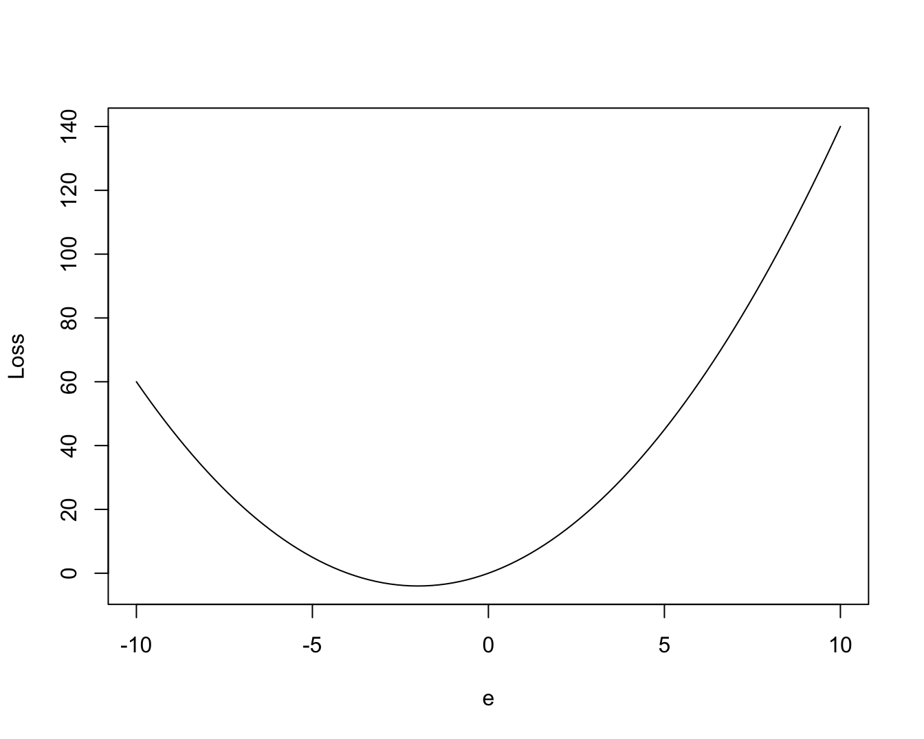
Figure 1.7: Asymmetric Loss Function

Once we have chosen our loss function, the optimal forecast can be obtained by minimizing the expected loss function.

An optimal forecast minimizes the expected loss from the forecast, given the information available at the time. Mathematically, we denote it by \(f^*_{t,h}\) and it solves the following minimization problem: \[\begin{equation} min_{f_{t,h}} E(L(e_{t,h})|\Omega_t) \end{equation}\]

In theory we can assume any functional form for the loss function and that will lead to a different optimal forecast. An important result that follows from a specific functional form is stated as Theorem 1.1.

Theorem 1.1 If the loss function is quadtratic then the optimal forecast is the conditional mean of the time series of interest. Formally, if \(L(e_{t,h})=e_{t,h}^2\) then, \[\begin{equation} f^*_{t,h}=E(y_{t+h}|\Omega_t) \end{equation}\]

Note that \(E(e_{t,h}^2)\) is known as mean squared errors (MSE). Hence, the expected loss from a quadratic loss function is the same as the MSE. In this course, we assume that the forecaster faces a quadratic loss function and hence based on Theorem 1.1, we will learn different models for estimating the conditional mean of the future value of the time series of interest, i.e., \(E(y_{t+h}|\Omega_t)\).