A Review of Serial Correlation and Heteroscedasticity
A.1 Classical Assumptions
Similar to our discussion in chapter 2, a desirable sample estimator must be unbiased and efficient. The discussion so far has focused on estimating regression parameters using sample data on the dependent and the independent variables. We will now focus on the conditions under which the OLS estimator of regression parameters are unbiased and efficient.
Suppose we have the following regression model:
\[Y_i = \beta_0 + \beta_1 X_i+ \epsilon_i\]
In the above model, \(\beta_0\) and \(\beta_1\) denote true but unknown population parameters of interest. We can use a sample data for \(Y_i\) and \(X_i\) to compute sample estimators for these two parameters. OLS is one such method of obtaining sample estimators \(\hat{\beta_0}\) and \(\hat{\beta_1}\). For these OLS estimators to be unbiased and efficient we need:
- Unbiasedness:
\[E(\hat{\beta_0)}=\beta_0 \ \text{and} \ E(\hat{\beta_1)}=\beta_1\]
- Efficiency:
\[Var(\hat{\beta_0}) \ \text{and} \ Var(\hat{\beta_1}) \ \text{are smallest possible.} \]
In order for the OLS estimators to be unbiased and efficient, we need a set of assumptions to be satisfied. These assumptions are known as classical assumptions and the result is formally known as the Gauss-Markov theorem named after two mathematicians, namely, Carl Gauss and Andrey Markov.
Theorem A.1 (Gauss-Markov theorem) The OLS estimator is the best linear and unbiased estimator (BLUE) if and only if the following six classical assumptions are satisfied:
The regression model is linear in parameters.
There is no linear relationship between included independent variables in the regression model or there is no perfect multicollinearity.
The expected value of the regression error term is 0.
\[E(\epsilon_i)=0 \ \text{for all} \ i\]
- There is no heteroscedasticity, i.e, the variance of the regression error term is constant.
\[Var(\epsilon_i)=\sigma^2 \ \text{for all} \ i\]
- There is no serial correlation. In time series data serial correlation implies observations of a variable are correlated over time. This is also known as auto-correlation. One of the classical assumption is that there is no serial (or auto) correlation in regression error terms.\[Cor(\epsilon_t, \epsilon_{t-s})=0 \ \text{where} \ t\neq s\]
- No endogeneity problem, i.e, all included independent variables in the model are exogenous and hence are uncorrelated with the regression error terms.
\[Cor(X_{ki}, \epsilon_i) = 0 \ \text{for} k=1,2,3, .., K\ \]
Of these 6 assumptions, in practice, we often take assumptions 1 through 3 for granted and do not consider violations of these assumptions in our data. However, assumptions 3 to 6 are often not met in data and are investigated much more rigorously. Accordingly, in this chapter we will focus on heteroscedasticity, serial correlation, and no endogeneity.
A.2 Heteroscedasticity
One of the main assumptions that affect the efficiency of the OLS estimator is the assumption of no heteroscedasticity which forces a constant variance for the error term in our regression model. Consider the following simple regression model that explains food expenditure (\(Y\)) based on a person’s disposable income (\(X\)):
\[Y_i=\beta_0 + \beta_1 X_i + \epsilon_i\]
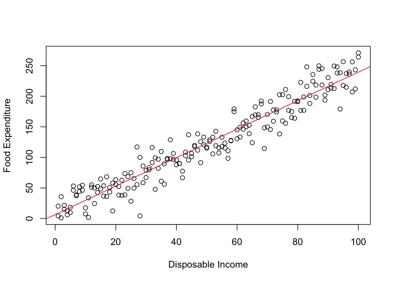
The classical assumption of no heteroscedasticity (or Homoscedasticity) implies that \(Var(\epsilon_i)=\sigma^2_\epsilon\). In the context of our example, this assumption can be interpreted as follows. The information a person’s income has for his food expenditure does not vary by the any characteristic of this person (say income). As a result the range of errors we can make in predicting someone’s food expenditure based on their income stays constant. Graphically, if error term are homoscedastic then there is no relationship between the range of errors we can make and a person’s income. Graphically, Figure 6.1 below shows this pattern–whether we look at observations with low income or those with high income, the range of errors we make is more or less constant.

Figure A.1: Homoscedastic Errors
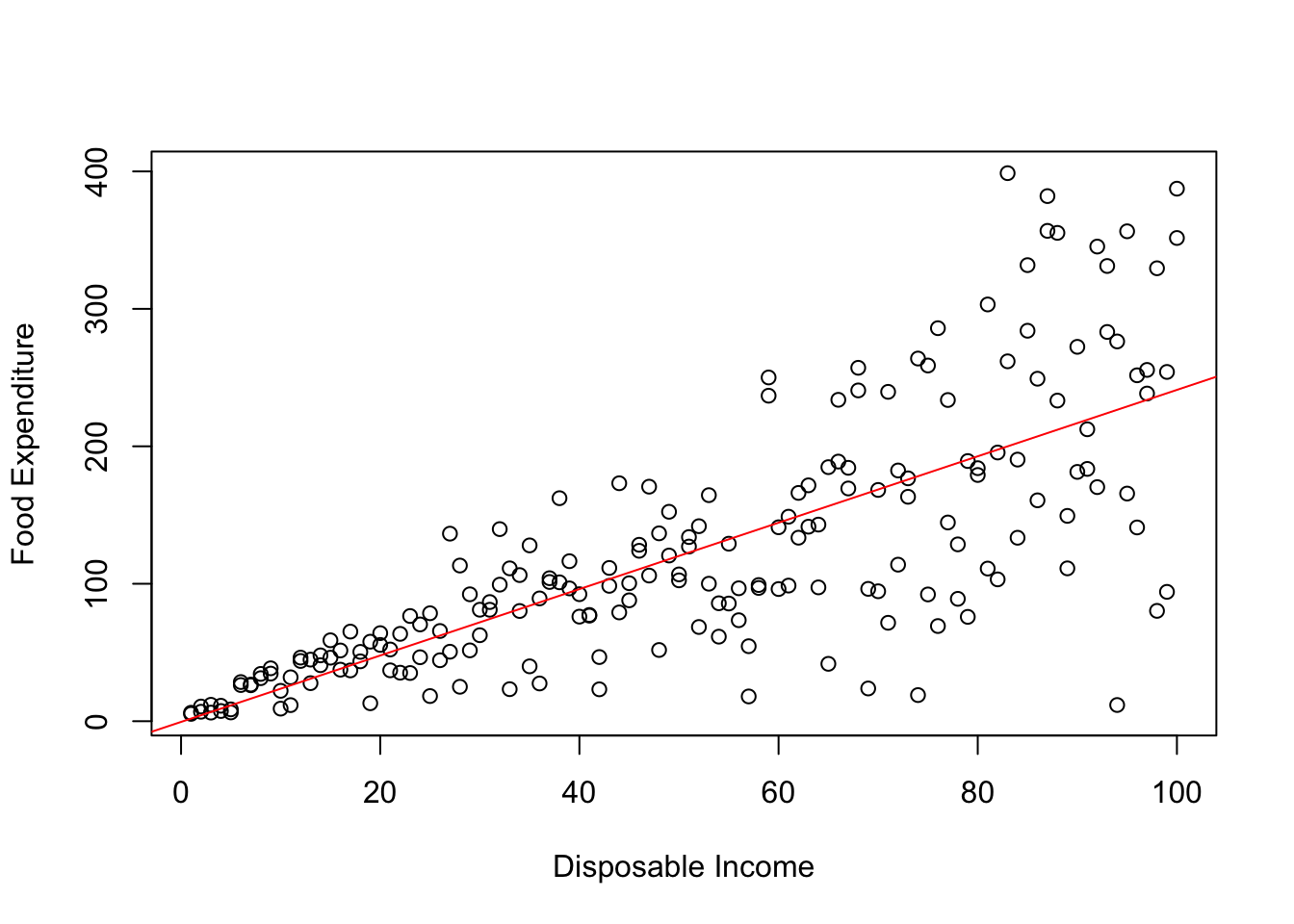
However, it is reasonable to argue that the value of information differ across observations in the following sense. Some observations have a greater role in reducing error variance than others. In our example, one can argue that food expenditure forms a bigger percent of a person with lower income than one with higher income who may use his income for non-food expenditure activities. In this case we would expect that the variance of errors will increase as income increases. This particular pattern of heteroscedastic errors is shown in Figure 6.2 below.

Figure A.2: Heteroscedastic Errors
In general the exact form of heteroscedasticity will depend on the nature of the problem at hand. However, whether or not heteroscedasticity is present in our data is an empirical question.
A.2.1 Consequences of Heteroscedasticity for the OLS estimator
Presence of heteroscedasticity is a violation of the classical assumption and accordingly will affect the properties of the OLS estimator. In general, if there is heteroscedasticity in data then:
The OLS estimator of each \(\beta\) coefficient is still unbiased.
However, due to ignoring the systematic variation in the error term, the OLS estimator is no longer efficient and the sample estimators of the standard errors of each \(\beta\) is incorrect. Consequently, we cannot conduct hypothesis testing on regression coefficients using the OLS estimator.
A.3 Testing for Hetroscedasticity in data
The first step for incorporating heteroscedasticity in our estimation is to test for its presence in our sample data. This test is based on OLS residuals of the original regression model and accounts for both linear and non-linear forms of heteroscedasticity. Consider the following regression model with two independent variables:
\[Y_i=\beta_0 + \beta_1 X_{1i} + \beta_2 X_{2i} + \epsilon_i\]
Using OLS we can obtain the residuals from this model, denoted by \(e_i\). Next, we will use this residual data to test for the presence of heteroscedasticity.
A.3.1 LM test for linear heteroscedasticity: BP test
The first test of heteroscedasticity is the Breusch-Pagan (BP) test of linear heteroscedasticity. The procedure for implementing this test is detailed below:
Step 1. Estimate the regression model using OLS and obtain residuals: \(e_i\)
Step 2: Estimate the BP regression model where the dependent variable is squared residuals and all independent variables are included on the right hand side:
\[e^2_i=\alpha_0 + \alpha_1 X_{1i} + \alpha_2 X_{2i} + \epsilon_i\]
Obtain \(R^2\) from this regression and denote it by \(R^2_{BP}\).
Step 3: The test of linear Heteroscedasticity is given by-
\[H_0: \alpha_1=\alpha_2=0 \Rightarrow \text{No linear heteroscedasticity}\] \[H_A: Not \ H_0 \Rightarrow \text{linear heteroscedasticity}\]
The test statistic id denoted by \(LM\) and the formula is given by:
\[LM=R^2_{BP} \times N\]
where \(N\) denotes sample size. Under the null hypothesis this test statistic follows Chi-square distribution with \(J\) degrees of freedom, where \(J\) denotes number of independent variables in the BPG regression of Step 2. If the LM test statistic is greater than the critical value from the Chi-square distribution, we reject the null hypothesis and conclude that there is sample evidence for linear heteroscedasticity.
A.3.2 LM test for linear heteroscedasticity: White’s test
We can also test for the presence of non-linear heteroscedasticity using White’s test. The procedure for implementing this test is detailed below:
Step 1. Estimate the regression model using OLS and obtain residuals: \(e_i\)
Step 2: Estimate the BPG regression model where the dependent variable is squared residuals. Now, independent variables include all independent variables, squared of all independent variables, and their product. So for example with 2 independent variables \(X_1\) and \(X_2\) we get the following White regression:
\[e^2_i=\alpha_0 + \alpha_1 X_{1i} + \alpha_2 X_{2i} + \alpha_3 X^2_{1i} + \alpha_4 X^2_{2i}+\alpha_5 (X_{1i}\times X_{2i})+ \epsilon_i\]
Obtain \(R^2\) from this regression and denote it by \(R^2_{White}\).
Step 3: The test of Hetroscedasticity is given by-
\[H_0: \alpha_1=\alpha_2=\alpha_3=\alpha_4=\alpha_5=0 \Rightarrow \text{No heteroscedasticity}\] \[H_A: Not \ H_0 \Rightarrow \text{heteroscedasticity}\]
The test statistic id denoted by \(LM\) and the formula is given by:
\[LM=R^2_{White} \times N\]
where \(N\) denotes sample size. Under the null hypothesis this test statistic follows Chi-square distribution with \(J\) degrees of freedom, where \(J\) denotes number of independent variables in the White regression of Step 2. If the LM test statistic is greater than the critical value from the Chi-square distribution, we reject the null hypothesis and conclude that there is sample evidence for heteroscedasticity.
Example A.1 (Testing for Hetroscedasticity) One of the most important models in finance is the Fama-French 3-factor model of risk premium of a stock. As per this model, the expected return on an asset over and above a risk free rate depends on depends on three factors:
Market risk: Market return minus risk free rate
Size premium: small market captilization stocks tend to out perform large market capitalization stocks. This variable captures this permium.
Value premium: Stocks with high book-to-market value out perform those with low value. This variable in this sense captures the value premium.
The regression model implied is given by:
\[y_t= \beta_0 + \beta_1 X_{1t} + \beta_2X_{2t} + \beta_3 X_{3t} + \epsilon_t\]
Here, \(y_t\) is the return on a stock minus the risk free rate. In this example we will use IBM stock and proxy risk free rate by using return on 1 month TB. \(X_{1t}\) denotes market risk, \(X_{2t}\) denotes size premium, and \(X_{3t}\) denotes value risk. The data for these three factors is downloaded from the following website:
https://mba.tuck.dartmouth.edu/pages/faculty/ken.french/data_library.html
In this application we use monthly data from Jan-2007 through June 2019. Table A.1 provides the estimation of this model using OLS.
| Dependent variable: (Return on IBM-Risk Free Rate) | ||||
|---|---|---|---|---|
| Explanatory Variables | b | s.e.(b) | t-ratio | p-value |
| Intercept | -0.054 *** | 0.010 | -5.245 | <0.001 |
| Market Risk Premium | 0.014 *** | 0.002 | 6.083 | <0.001 |
| Size Premium | 0.006 | 0.007 | 0.851 | 0.396 |
| Volume Premium | -0.012 | 0.006 | -1.943 | 0.054 |
| Observations | 150 | |||
| R2 / R2 adjusted | 0.215 / 0.199 | |||
| log-Likelihood | 101.354 | |||
|
||||
In order to use the OLS estimator for hypothesis testing, we need to confirm whether there is heteroscedasticity in our data. For this example the BP test regression is given by:
\[e^2_i=\alpha_0 + \alpha_1 f_{1i} + \alpha_2 f_{2i} +\alpha_3 f_{3i} + \epsilon_i\]
The null hypothesis for no heteroscedasticity requires \(\alpha_1=\alpha_2=\alpha_3=0\).
The White test regression is given by:
\[e^2_i=\alpha_0 + \alpha_1 f_{1i} + \alpha_2 f_{2i} +\alpha_3 f_{3i} + \alpha_4 f^2_{1i} +\alpha_5 f^2_{2i} + \alpha_{6}f^2_{3i} + \alpha_7 (f_{1i} \times f_{2i})+ \alpha_8 (f_{1i} \times f_{3i})+ \alpha_9 (f_{2i} \times f_{3i})+\epsilon_i\]
The null hypothesis for no heteroscedasticity requires \(\alpha_1=\alpha_2=\alpha_3=\alpha_4=\alpha_5=\alpha_6=\alpha_7=\alpha_8=\alpha_9=0\). We conduct both BP and White’s test in R and present the results in Table A.2. We find that there is evidence of heteroscedasticity according to both tests, as we reject the null hypothesis for BP test at 5% level of significance and we reject the null hypothesis for White’s test at 10% level of significance.
| BP test | White’s test | |
|---|---|---|
| LM statistic | 10.099 | 15.396 |
| p-value | 0.018 | 0.081 |
A.4 Serial correlation
In time series data it is common to observe correlation across observations over time. Indeed many relationships in economics are dynamic in nature. For example, consumption habits indicate past consumption has an effect on current consumption. Similarly, production activities typically stretch over multiple periods and output in one period is often affect by the level produced in the previous period. As these examples indicate it is reasonable to argue that time series economic data may exhibit some kind of serial correlation.
The correlation between observations of a time series variable is captured by the autocorrelation function (ACF) which is given by:
\[ACF(s)=\frac{Cov(y_t, y_{t-s})}{\sigma_{y_t} \times \sigma_{y_{t-s}}}\]
Note that here \(t\) indexes the current period and \(s\) is an integer. For example, if \(s=1\), we are looking at correlation between \(y_{t}\) and \(y_{t-1}\). This is known as first order serial correlation. Similarly, for \(s=2\), we get the second order serial correlation between \(y_{t}\) and \(y_{t-2}\). In this ACF is a function of \(s\) and will give us a series of values of correlation of the current period with \(s\) past periods.
One of the main assumptions that affect the efficiency of the OLS estimator is the assumption of no serial correlation which forces the error term in our regression model to be independent across observations over time. Consider the following simple regression model:
\[Y_t=\beta_0 + \beta_1 X_t + \epsilon_t\]
The classical assumption of no serial correlation implies that \(Cor(\epsilon_t,\epsilon_{t-s})=0\), where \(t\) indexes current time period and \(s\) is an integer.
However, it is quite possible that the regression errors are actually correlated over time. For simplicity, lets assume that the error term in our model has first order serial correlation of the following form:
\[\epsilon_t = \rho \epsilon_{t-1} + u_t\]
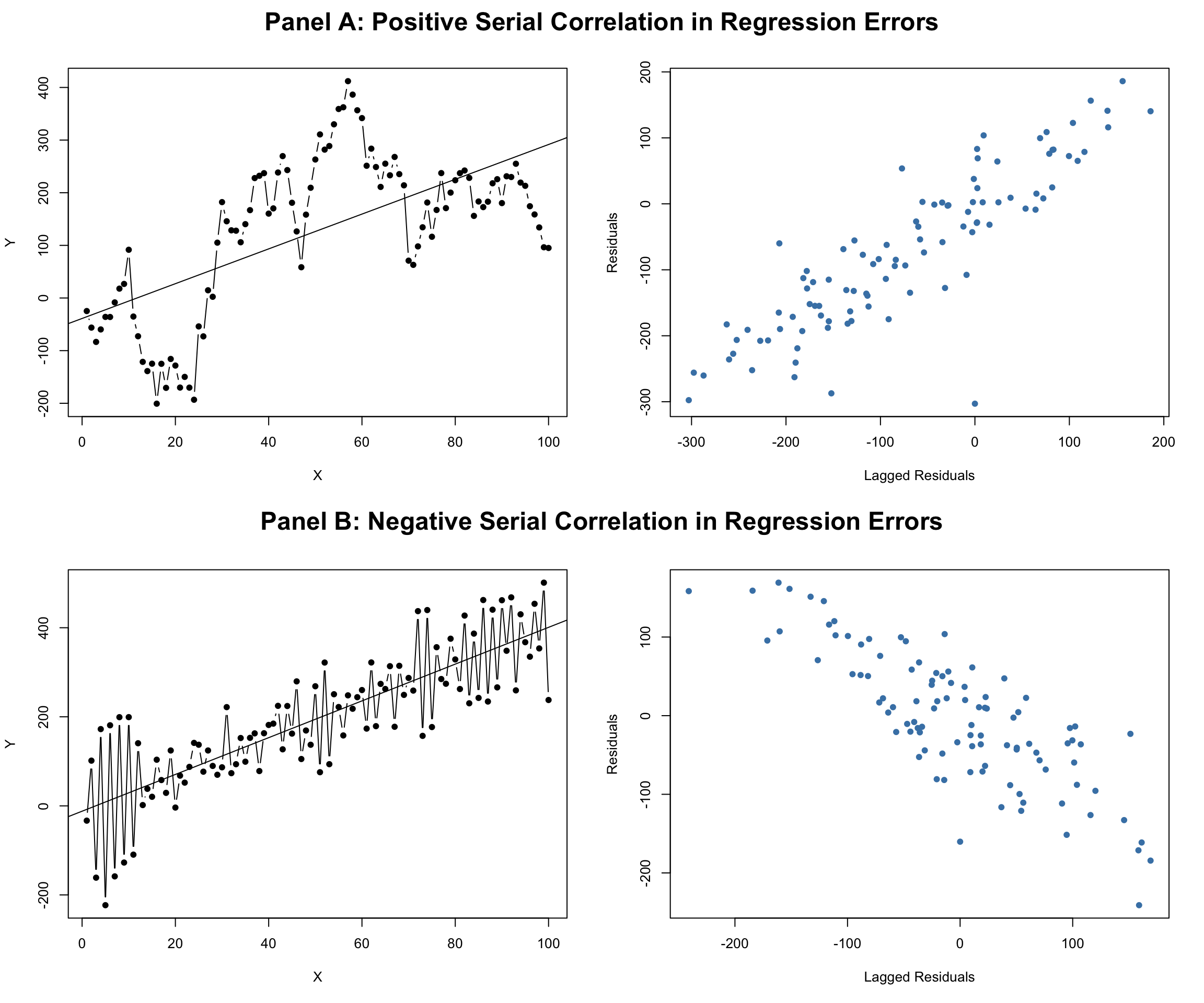
Here \(\rho\) captures the first order serial correlation and is the slope parameter. \(u_t\) is a classical error term that satisfies all classical assumptions and hence is serially uncorrelated by definition. Now, depending on the sign of \(\rho\) the serial correlation can be positive or negative. In economics it is most common to observe positive serial correlation where the persistence in data ensures that a positive (negative) value of the regression error in one period is likely to be followed by another positive (negative) value. In contrast for negative serial correlation a positive error in one period is more likely to be followed by a positive error next period, and vice-versa. Figure A.3 below shows the pattern of residuals for the two cases of positive and negative serial correlation in the regression error terms.

Figure A.3: Serially correlated Errors
In general we can have higher order serial correlation in data and whether or not there is such correlation in our data is an empirical question.
A.4.1 Consequences of Serial Correlation for the OLS estimator
Presence of serial correlation is a violation of the classical assumption and accordingly will affect the properties of the OLS estimator. In general, if there is serial correlation:
The OLS estimator of each \(\beta\) coefficient is still unbiased.
However, the OLS estimator is no longer efficient and the sample estimators of the standard errors of each \(\beta\) is incorrect. Consequently, we cannot conduct hypothesis testing on regression coefficients using the OLS estimator.
A.5 Testing for Serial Correlation in data
A.5.1 Breusch-Godfrey (BG) LM test for serial correlation
In order to test for higher order serial correlations we can use the BG test which uses the OLS residuals to test for evidence of serial correlation. The procedure for this test is described below:
Step 1. Estimate the regression model using OLS and obtain residuals: \(e_t\)
Step 2: Estimate the BG regression model where the dependent variable is the residuals and independent variables are all X variables in the model, and lagged values of this residual. The number of lagged residuals capture the order of serial correlation. In general for testing serial correlation up to order of \(p\), we will estimate the following regression:
\[e_t=\alpha_0 + \gamma_1 c\cdot X_{1t}+ \gamma_2 \cdot X_{2t}+...+\gamma_K \cdot X_{kt}+ \alpha_1 e_{t-1} + \alpha_2 e_{t-2} +...+ \alpha_p e_{t-p} + u_t\]
Denote \(R^2_{BG}\) as the R-squared of this regression model.
Step 3: The serial correlation test is given by:
\[H_0: \alpha_1=\alpha_2=\alpha_3=....=\alpha_p=0\] \[H_A: Not \ H_0\]
The LM test statistic is given by:
\[LM=N\times R^2_{BG}\]
Under the null hypothesis, this test statistic follows Chi-square distribution with \(p\) degrees of freedom. If LM statistic is bigger than the critical value, we reject the null and conclude that there is serial correlation.
Example A.2 (Testing for serial correlation) Let us use the same example as the one we used for testing hetroscedasticity. We estimated a three factor model for the stock return of Apple using use monthly data from Jan-2007 through June 2019 (see Table A.1 for OLS estimation results of this model).
We can implement both tests for serial correlation in R using the lmtest package. Table A.3 below presents the results test-statistic for both serial correlation tests. For comparison, I am testing for first order serial correlation. the BG test clearly indicates presence of serial correlation as indicated by a p-value which is less than 0.05. For Durbin-Watson test, sample size is 150 and K=3. Using the Durbin-Watson table we get dL=1.584 and dU=1.665. Because d=0.75 is less than dL, we reject the null hypothesis of no serial correlation and conclude there is evidence for positive first order serial correlation.
| BG test | |
|---|---|
| Test statistic | 53.623 |
| p-value | 0.000 |