Chapter 7 Vector Autoregression (VAR) Model
Thus far our analysis has been limited to a univariate time series. Often one maybe interested in understanding the dynamics of multiple time series variables. Vector Autoregression (VAR) model is one of the most commonly used model for this purpose. Suppose you have \(N\) time series variables in your sample Then a VAR model is a system of \(N\) linear equations where each variable is modeled as a linear function of its own lags and current and past values of the remaining \(N-1\) variables. In this sense a VAR model combines and extends the the AR model and distributed lag model we covered earlier.
There are two main ways we can specify a VAR model, each distinguished by the treatment of contemporaneous effects among variable included in the model. To make each type’s main features salient, suppose that we have three variables in our model: inflation (denoted by \(\pi\)), unemployment (denoted by \(u\)), and the federal fund rate (denoted by \(i\)). In the remainder of this chapter will use this 3-variable system as our example.
7.1 Reduced-form VAR
In a reduced-form VAR we abstract away from any contemporaneous linkages among variables in the model and hence in that sense take an atheoretical approach to estimating dynamic relationships among these variables. Specifically, we assume that each variable in the model is a function of its own lags and lags of remaining variables in the system. For example, using our 3 variables, a reduced-form VAR(1) is given by:
\[\pi_t = a_{10} + a_{11} \pi_{t-1} + a_{12} u_{t-1} + a_{13} i_{t-1} + e_{1t}\] \[u_t = a_{20} + a_{21} \pi_{t-1} + a_{22} u_{t-1} + a_{23} i_{t-1} + e_{2t}\] \[i_t = a_{30} + a_{31} \pi_{t-1} + a_{32} u_{t-1} + a_{33} i_{t-1} + e_{3t}\]
Note that:
The above system of 3-equations can easily be estimated as it only includes lagged data for each variable as independent variable, which by definition is pre-determined. Hence, we can estimate each equation separately by OLS.
In the above example we use 1 lag for simplicity. In practice the number of lagged values to include in each equation can be determined using AIC or BIC.
Each equation will provide a forecast for that particular variable. Hence, in our example we can generate forecasts for all three variables in our model.
One important drawback of the reduced-form VAR is that it cannot be used for structural inference and policy analysis. For example, suppose we are want to find out what will be the effect of raising the ffr by 50 basis points on inflation and unemployment? To answer this question, we need the shocks in each equation to be independent of each other. Only then, for example, we can say that \(e_{3t}\) represents shock to the FFR alone. However, in the reduced-form VAR, because each variable is related to each other, shocks in each equation are also correlated to each other.
7.2 Structural VAR
The reduced-form VAR specified above is atheoretical in the sense that it does not impose any economic structure on the relationships between different variables. As a result a reduced-form model cannot be used to uncover causal relationships between correlated variables. A structural VAR model allows each variable to depend on past as well as current values of other variables in the system. As a result, a structural VAR adds contemporaneous linkages among variables included in the model. Continuing with our example, a structural version of the 3-variable VAR can be written as follows:
\[\pi_t = \beta_{11} + \beta_{12} u_t + \beta_{13} i_t + \phi_{11} \pi_{t-1} + \phi_{12} u_{t-1} + \phi_{13} i_{t-1} + \epsilon_{1t}\] \[u_t = \beta_{21} + \beta_{22} \pi_t+ \beta_{23} i_t+\phi_{21} \pi_{t-1} + \phi_{22} u_{t-1} + \phi_{23} i_{t-1} + \epsilon_{2t}\] \[i_t = \beta_{31} + \beta_{32}\pi_t + \beta_{33}u_t+ \phi_{31} \pi_{t-1} + \phi_{32} u_{t-1} + \phi_{33} i_{t-1} + \epsilon_{3t}\]
There are three key things to note here:
In each equation we now have contemporaneous linkages among variables. For example, in the first equation, \(\beta_{12}\) and \(\beta_{13}\) capture the effect of changes in period \(t\) values of unemployment and ffr on the period \(t\) value of inflation.
By definition the error terms are uncorrelated across equations and hence each error term can be interpreted as representing a pure shock to that particular variable. For example, \(\epsilon_{3t}\) represents shocks to the ffr often caused by the monetary policy actions of the Fed.
OLS estimation of each equation separately would provide biased estimates as there is a simultaneity bias inherent in the specification of the structural VAR. For example, in the inflation equation, inflation depends on current period unemployment and interest rate. But, in the unemployment equation, unemployment depends on current period inflation and interest rate as well. This kind of reverse causality causes OLS estimator to be biased.
Consequently, a structural VAR model cannot be estimated using OLS. In order to process we need to impose some kind of identifying restrictions on the structural VAR model to deal with the contemporaneous linkages among variables. Such restrictions often come from economic theory and may involve the entire model or a just a single equation. However, to conduct structural inference we have to use economic theory to afford structural interpretation to shocks of our VAR model.
7.3 Cholesky Decomposition and Recursive VAR model
One solution that falls in between the reduced-form VAR with no structural interpretation and the structural VAR with full set of contemporaneous linkages is the recursive VAR model. In this specification, the error term in each equation is assumed to be uncorrelated with the error term in the preceding equations. This is accomplished by assuming some sort of ordering among variables in the VAR model so that only some variables contemporaneously affect others. For example, suppose we use the following ordering: inflation, unemployment, and the federal fund rate (ffr). This ordering will imply the following recursive VAR model:
\[\pi_t = \beta_{11} + \phi_{11} \pi_{t-1} + \phi_{12} u_{t-1} + \phi_{13} i_{t-1} + \epsilon_{1t}\] \[u_t = \beta_{21} + \beta_{22} \pi_t+\phi_{21} \pi_{t-1} + \phi_{22} u_{t-1} + \phi_{23} i_{t-1} + \epsilon_{2t}\] \[i_t = \beta_{31} + \beta_{32}\pi_t + \beta_{33}u_t+ \phi_{31} \pi_{t-1} + \phi_{32} u_{t-1} + \phi_{33} i_{t-1} + \epsilon_{3t}\]
Note that:
The ordering we assumed: inflation, unemployment, and ffr, implies that the first variable (inflation) has no contemporaneous linkage with unemployment and ffr. The second variable (unemployment) is affected by contemporaneous inflation and the third variable (ffr) is affected by both contemporaneous inflation and unemployment. The main implication of this ordering is that \(cor(\epsilon_{1t},\epsilon_{2t})=0\), \(cor(\epsilon_{2t},\epsilon_{3t})=0\), and \(cor(\epsilon_{1t},\epsilon_{3t})=0\).
In practical implementations of the recursive VAR model, it is common to first estimate the reduced-form VAR model using OLS for each equation separately. Then, we decompose the covariance matrix to reduced-form residuals using Cholesky decomposition method to obtain uncorrelated error structure consistent with the recursive VAR model specified above. This can be used to investigate how shocks to one variable affect other variables in the system.
If we change the ordering, we will get different results. In a model with \(N\) variables, there are N! possible orderings. So in our example, there are 3!= 6 possible alternative specifications for the VAR model. Hence, this approach requires us to judiciously choose the ordering of the variables.
7.4 Impulse Response Function, Forecast Error Variance Decomposition, and Granger Causality
In addition to estimating each equation and providing a forecast of all variables in the system, there are two additional outputs produced by a VAR model which can be used for both descriptive and inference purposes. This analysis requires us to either use a recursive VAR model or impose some restrictions based on economic theory so that each shock can be interpreted as a shock to that particular variable. In this chapter we will use the recursive VAR structure when discussing impulse response functions and variance decomposition.
7.4.1 Impulse response function
Suppose we are interested in finding out how shock to one variable in the system at time \(t\) affects the dynamics of other variables. For example, suppose there is unanticipated increase in the ffr caused by the actions of the Fed. What would be the dynamic response of inflation and unemployment to this monetary policy shock? Using the recursive VAR, we can interpret the shock to the FFR (the last variable in our ordering) as a pure interest rate shock because it is by construction uncorrelated with shocks to inflation and unemployment. The impuse response produced by the VAR model traces out the response of current and future values of unemployment and inflation to one-unit increase in the error term of the ffr equation, holding error terms in inflation and unemployment equation at zero. We can study both the impact effect as well as the cumulative effect of such a shock to ffr on unemployment and inflation.
7.4.2 Forecase Error Variance Decomposition
Another useful output from an estimated VAR model is the forecast error variance decomposition (fevd). Here, we can address the following question: following a shock to one of the variables in the VAR model what percentage of the variance in the forecast error of other variables in the model can be attributed to this particular shock? For example, what percentage of the forecast error variance of inflation can be attributed to the shock in inflation, shock in unemployment, and shock to ffr. In this sense the forecast error variance decomposition measures the amount of each variable in the VAR model contributes to the other variables in the autoregression.
7.4.3 Granger causality
Another important analysis that one can conduct using a VAR model is Granger-causality. As a bi-variate concept, Granger causality means that lags of one variable improves our capacity to predict another variable. For example, if unemployment Granger-causes inflation, then lags of unemployment have non-zero coefficients in the reduced-form inflation equation. Formally, consider the following regression:
\[\pi_t=\beta_0 + \sum_{i=1}^{P} \beta_i u_{t-i} \sum_{i=1}^{P} \delta_i \pi_{t-i} + \epsilon_t\]
To test whether unemployment Granger causes inflation we can conduct the following hypothesis test:
\[H_0: \beta_1=\beta_2=...=\beta_p=0\] \[H_A: \text{Not} \ H_0\]
This is an F-test and rejection of the null hypothesis indicates unemployment Granger-causes inflation.
7.5 Application: Effect of monetary policy on inflation and unemployment
The Federal reserve bank (The Fed) in the U.S. has a dual mandate: to maintain low inflation and low unemployment. The monetary policy stance of the Fed is expressed in terms of the federal funds rate (ffr). In this section we learn how to estimate a VAR model with three variables: inflation (\(\pi_t\)), unemployment (\(u_t\)), and interest rate (\(i_t\)). For this purpose we will use quarterly data on these variables from 1960Q1 through 2019Q2. We will use the Fred Stat website and download data on these variables:
- Seasonally quarterly GDP deflator (GDPDEF): https://fred.stlouisfed.org/series/GDPDEF ht We define inflation as follows:
\[\pi_t = 400 \times ln\left(\frac{P_t}{P_{t-1}} \right)\]
Here \(P_t\) denotes GDP deflator for quarter \(t\).
Seasonally adjusted Civilian unemployment rate (UNRATE): https://fred.stlouisfed.org/series/UNRATE
Effective federal funds rate (FEDFUNDS): https://fred.stlouisfed.org/series/FEDFUNDS
The first step in any VAR analysis is to ensure that all variables in the model are stationary. Although not reported here, I find that inflation is stationary whereas unemployment and interest rate are first difference stationary. Accordingly, we will use inflation and first differences of unemployment and interest rate in our VAR analysis. The second step in the VAR analysis is to determine the optimal number of lags. Table 7.1 presents different information criteria for up to 8 lags. Using SC criterion we select optimal lags to be 2.
Hence, our reduced-form VAR model is given by:
\[ \pi_t = a_{10} + a_{11} \pi_{t-1} + a_{12} u_{t-1} + a_{13} i_{t-1} + b_{11} \pi_{t-2} + b_{12} u_{t-2} + b_{13} i_{t-2} + e_{1t}\] \[ u_t = a_{20} + a_{21} \pi_{t-1} + a_{22} u_{t-1} + a_{23} i_{t-1}+ b_{21} \pi_{t-2} + b_{22} u_{t-2} + b_{23} i_{t-2} + e_{2t}\] \[ i_t = a_{30} + a_{31} \pi_{t-1} + a_{32} u_{t-1} + a_{33} i_{t-1}+ b_{31} \pi_{t-2} + b_{32} u_{t-2} + b_{33} i_{t-2}+ e_{3t}\]
We can estimate the above model using OLS for each equation separately. It is a common practice to report the variance decomposition and impulse response from an estimated VAR model instead of reported the estimated coefficients for each equation. I will follow that convention and only report the analysis based on the estimated VAR model. The table below shows the results of Granger-causality test using optimal lag of 2. We find that inflation Granger-causes ffr and unemployment as indicated by a low p-value for the null hypothesis of no Granger-causality. Similarly, unemployment Granger-causes inflation and ffr. Finally, ffr also Granger-cause other two variables.
##
##  Granger causality H0: inf do not Granger-cause u ffr
##
## data:  VAR object varmodel
## F-Test = 3.9185, df1 = 4, df2 = 738, p-value = 0.003718
##
## Granger causality H0: u do not Granger-cause inf ffr
##
## data: VAR object varmodel
## F-Test = 1.8588, df1 = 4, df2 = 738, p-value = 0.1158##
## Granger causality H0: ffr do not Granger-cause inf u
##
## data: VAR object varmodel
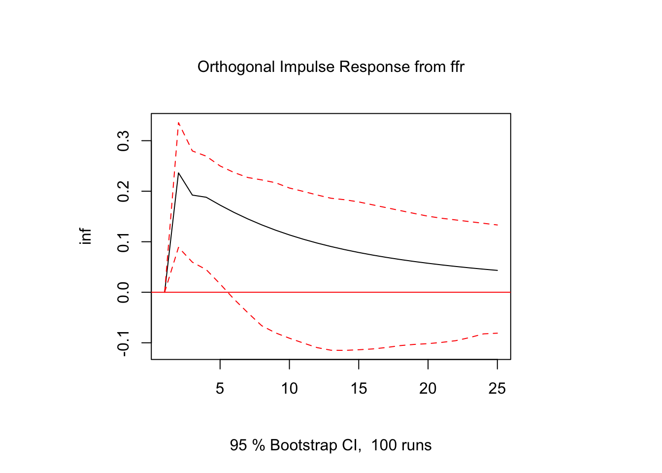
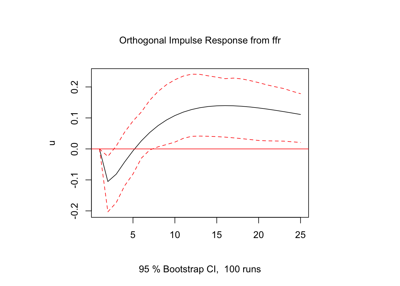
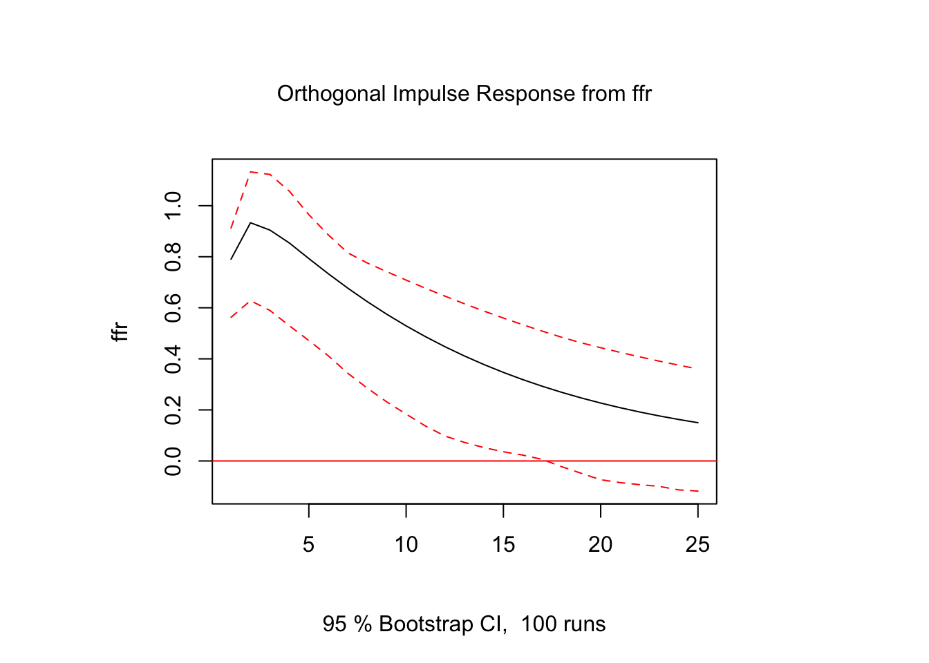
## F-Test = 5.2338, df1 = 4, df2 = 738, p-value = 0.0003679Next we present the impulse responses for the recursive VAR structure where we use the following ordering: inflation, unemployment, and interest rate. For brevity, I only show the effect of an unexpected increase in ffr on all three variables as this shock propagates through the recursive VAR structure using the estimated coefficients from the reduced-form VAR model. From Figures 7.1 through 7.3 we observe a persistent positive effect of higher interest rate on both unemployment and inflation that fades over time.

Figure 7.1: Impulse Response Function

Figure 7.2: Impulse Response Function

Figure 7.3: Impulse Response Function
Next we present the forecast error variance decomposition results that decomposes the variance in forecast error of a variable into own contribution and contribution of shocks to other variables. In Table below we show this analysis at 4 forecast horizons, namely, 1 period, 4 period, 8 period, and 12 periods. They suggest considerable interaction among the variables. For example, at the 12-quarter horizon, 63 percent of the forecast error variance in for ffr can be attributed to the inflation and unemployment shocks in the recursive VAR. In contrast, only 15 percent of the forecast error variance for inflation comes from shocks to ffr and unemployment.
| horizon | inf | u | ffr |
|---|---|---|---|
| 1 | 1.000 | 0.000 | 0.000 |
| 4 | 0.949 | 0.002 | 0.048 |
| 8 | 0.940 | 0.003 | 0.057 |
| 12 | 0.937 | 0.004 | 0.059 |
| horizon | inf | u | ffr |
|---|---|---|---|
| 1 | 0.077 | 0.923 | 0.000 |
| 4 | 0.070 | 0.916 | 0.014 |
| 8 | 0.068 | 0.918 | 0.015 |
| 12 | 0.062 | 0.902 | 0.037 |
| horizon | inf | u | ffr |
|---|---|---|---|
| 1 | 0.016 | 0.061 | 0.923 |
| 4 | 0.044 | 0.102 | 0.854 |
| 8 | 0.141 | 0.092 | 0.767 |
| 12 | 0.231 | 0.079 | 0.689 |
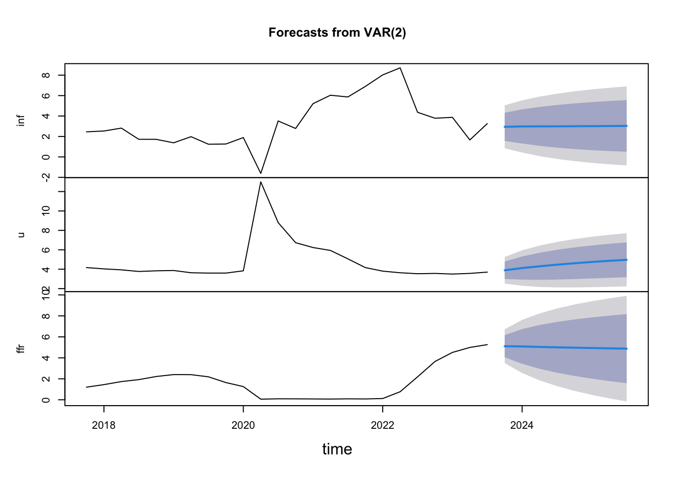
Finally, we can use our reduced-form VAR estimation to produce forecasts for each variable in the model. Figure 7.4 below provides forecast for next 8 quarters from 2019Q3 through 2021Q2. These forecasts can be compared with univariate forecast for each variable using ARIMA or some other method to assess the improvement in forecast accuracy due to estimating a VAR model.

Figure 7.4: Forecast for 2019Q3 through 2021Q2