Chapter 5 Modeling Trend and Seasonal Components
5.1 Trend Estimation
An important component of a time series is trend that captures the long run evolution of the variable of interest. There are two types of trends:
Deterministic Trend: the underlying trend component is a known function of time with unknown parameters.
Stochastic Trend: the trend component is random.
In this note we will focus on estimating and forecasting deterministic trend models. We will come back to stochastic trend later when we talk about stationarity property of a time series.
5.1.1 Parametrizing a deterministic trend
Whether or not there is deterministic trend in the data can be typically gleaned by simply plotting the time series over time. For example, Figure @ref(fig: ch5-figure1) below plots real GDP for the US at quarterly frequency. We can observe a positive time trend with real GDP increasing with time. In this section we will learn to fit a function that captures this relationship accurately.
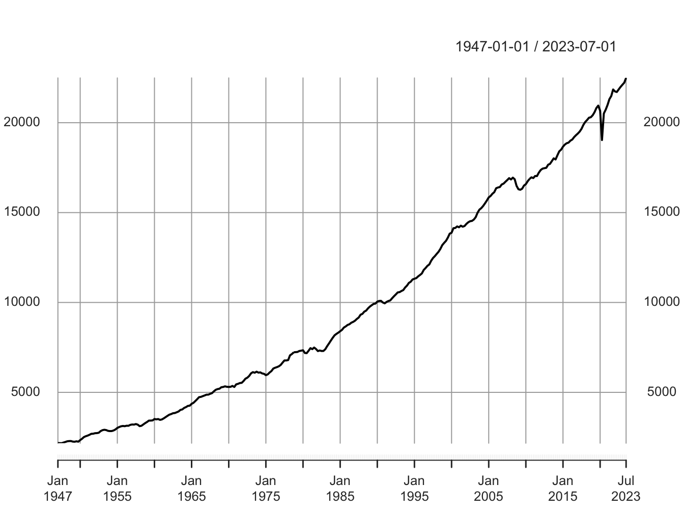
Figure 5.1: Real GDP (2012 Chained Billions of Dollars)
Note: The variable time is denoted by \(t\) and it is artificially created to take value of 1 for the first period, 2 for the second period and so on.
There are two commonly used functional forms for capturing a deterministic trend:
- Polynomial Trend: We fit a polynomial of appropriate order to capture the time trend. For example, A. Linear trend: \[\begin{equation} y_t=\beta_0 +\beta_1 t +\epsilon_t \end{equation}\]
B. Quadratic trend: \[\begin{equation} y_t=\beta_0 +\beta_1 t + \beta_2 t^2 +\epsilon_t \end{equation}\]
In general, we can fit a polynomial of order \(q\): \[\begin{equation} y_t=\beta_0 + \sum_{i=1}^q \beta_i t^i +\epsilon_t \end{equation}\]
We can estimate this model using the OLS. One of the key component here is to determine the right order of the polynomial. We can begin with a large enough number for \(q\) and then select the appropriate order using AIC or BIC criterion.
- Exponential or log-linear trend: In some cases we may want to use an exponential trend or equivalently a log-linear trend. \[\begin{align} y_t=e^{(\beta_0 +\beta_1 t +\epsilon_t)}\\ equivalently\\ log(y_t)=\beta_0 +\beta_1 t +\epsilon_t \end{align}\]
Again we can estimate the above model using OLS.
5.1.2 Uses of the Deterministic Trend Model
Once we have finalized our deterministic trend model i.e., either a polynomial of a specific order or log-liner trend, we can use the estimated model for the following two purposes:
Detrending our data: Suppose we would like to eliminate trend from our data. The residual from our final trend model is the detrended time series.
Forecasting: We can also forecast our time series based on the estimated trend. For example, suppose our final model is a quadratic trend. The predicted value is given by:
\[\begin{equation} \widehat{y_t}=\widehat{\beta_0}+\widehat{\beta_1} t + \widehat{\beta_2} t^2 \end{equation}\]
Then, the 1-period ahead forecast for \(y_{t+1}\) can be obtained by solving: \[\begin{equation} \widehat{y_{t+1}}=\widehat{\beta_0}+\widehat{\beta_1} (t+1) + \widehat{\beta_2} (t+1)^2 \end{equation}\]
5.1.3 Application: Estimating a polynomial trend for U.S. Real GDP
We will now fit a polynomial trend to the US real GDP data that was presented in Figure ??. We first estimate polynomials of different orders and select the optimal order determined by the lowest possible AIC/BIC. Table 5.1. shows these statistics for up to 4th order polynomial. We find that the lowest value occur at \(q=4\).
| order | AIC | BIC |
|---|---|---|
| 1 | 5191.926 | 5203.107 |
| 2 | 4489.932 | 4504.840 |
| 3 | 4457.576 | 4476.210 |
| 4 | 4420.521 | 4442.882 |
Hence, our final trend model is:
\[\begin{equation} y_t=\beta_0 +\beta_1 t + \beta_2 t^2 + \beta_3 t^3 + \beta_4 t^4 +\epsilon_t \end{equation}\]
The estimated trend model is presented in Table 5.2.
| Estimate | Std. Error | t value | Pr(>|t|) | |
|---|---|---|---|---|
| (Intercept) | 2037.755 | 93.220 | 21.860 | 0.000 |
| trend | 30.795 | 4.179 | 7.368 | 0.000 |
| I(trend^2) | -0.087 | 0.055 | -1.585 | 0.114 |
| I(trend^3) | 0.001 | 0.000 | 5.557 | 0.000 |
| I(trend^4) | 0.000 | 0.000 | -6.401 | 0.000 |
Using the estimated model, we can compute the detrended data as the residual and also forecast \(y_t\). Figure 5.2 below plots the detrended real GDP obtained as a residual from our trend model.
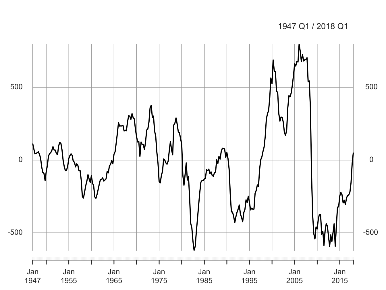
Figure 5.2: Detrended Real GDP
Figure 5.3 shows the forecast of real GDP for next 8 quarters along with the 95% confidence bands.
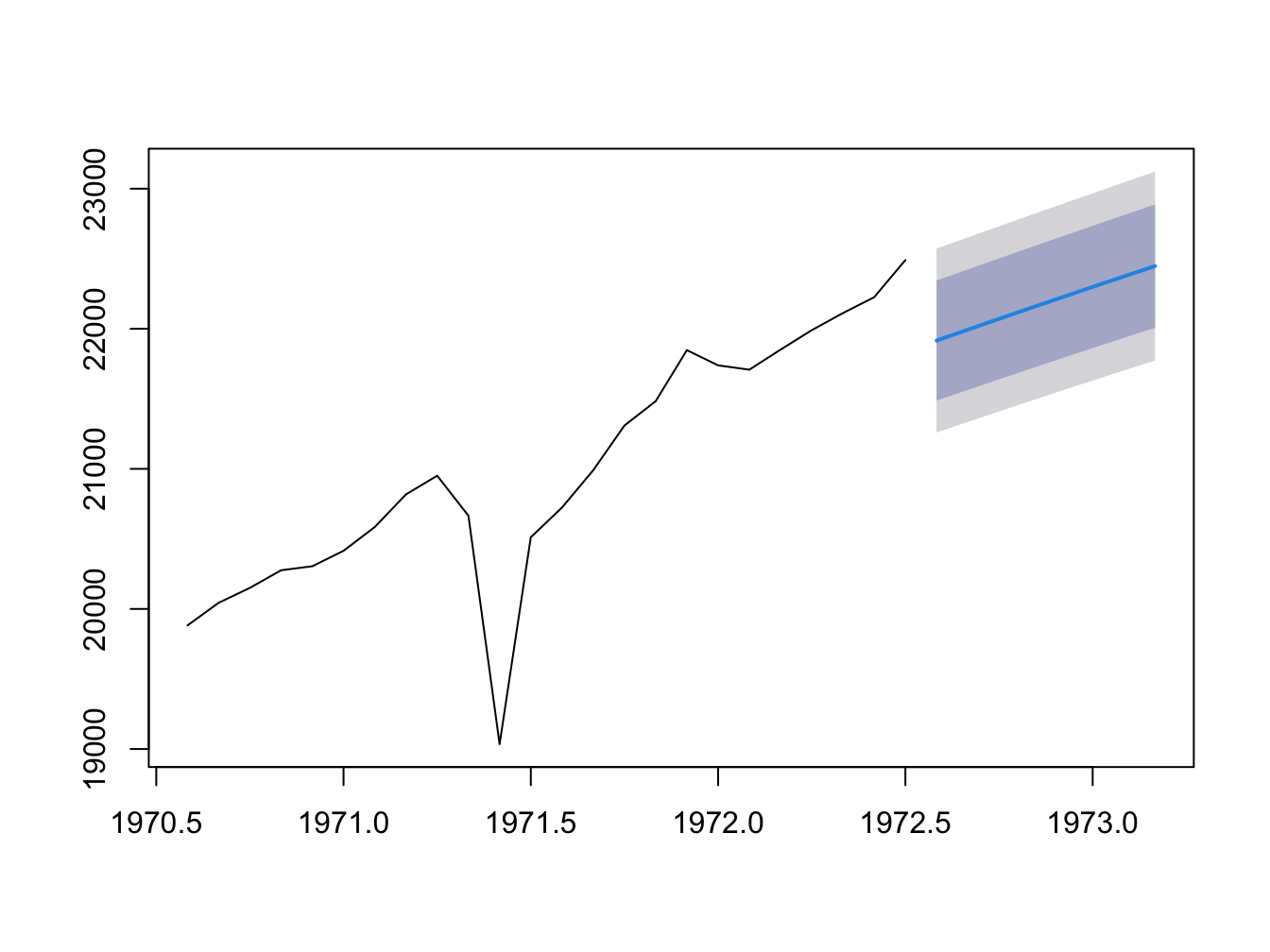
Figure 5.3: Forecast of Real GDP
5.2 Seasonal Model
We now focus on the seasonal component of a time series, i.e., that is periodic fluctuations that repeat themselves every season. For example, increase in ice cream sales during summer season. Just like trend component, such seasonal pattern could be deterministic or stochastic. In this chapter we will focus on estimating deterministic seasonal component.
In Figure 5.4 we plot housing starts in the U.S. The data is at monthly frequency and we can see a clear seasonal pattern. Housing starts seem to increase in spring and summer months. This is followed by a decline in fall and winter months.
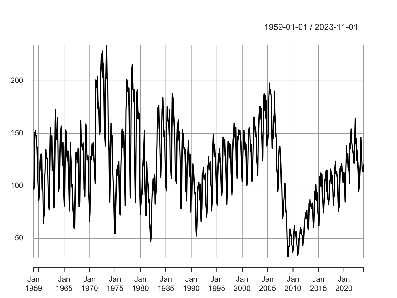
Figure 5.4: Housing Starts in U.S.
One option to deal with seasonality is to obtain seasonally adjusted data (or deseasonalized data) from the source itself. Alternatively, we can use decomposition method and appropriately filter out the seasonal component. However, if our objective is to explicitly model the seasonal component of a time series then we must work with non-seasonally adjusted data.
5.2.1 Regression Model with Seasonal Dummy Variables
One way to account for seasonal patterns in data is to add dummy variables for season. To avoid perfect multicollinearity, is there are \(s\) seasons, we can include \(s-1\) dummy variables. For example, for quarterly data, \(s=4\) and hence we need \(s-1=3\) dummy variables in our regression model. Formally, for quarterly data, the seasonal regression model is given by:
\[\begin{equation} y_t= \beta_0 + \beta_1 D_{1t}+ \beta_2 D_{2t} + \beta_3 D_{3t} + \epsilon_t \end{equation}\]
In the above regression model, \(D_1,D_2,\) and \(D_3\) are dummy variables that capture first three quarters of the year. For example, \(D_1=1\) for the first quarter and \(D_1=0\) otherwise. Similarly, \(D_2=1\) for the second quarter and \(D_2=0\) otherwise. In this example, we use the fourth quarter as the base group.
The above model can be estimated using OLS. Again, we can use the residual from our estimated model as a measure of deseasonlized data. We can also forecast the dependent variable based on the seasonal component only.
5.2.2 Application: Seasonal Model of Housing Starts
We now estimate a seasonal regression model for the housing starts data presented in Figure 5.4. The data is at monthly frequency which implies we can have 12 possible seasons and hence would need 11 dummy variables in our regression model. Formally, we use January as the base group and include dummy variables for the last 11 months of the year:
\[\begin{equation} y_t=\beta_0 + \sum_{i=2}^{12}\beta_i D_{it} + \epsilon_t \end{equation}\]
Table 5.3 presents the estimation results for this exercise. In Figure 5.5 we plot the forecast of housing starts for next 12 months using our estimated model, along with 95% confidence bands.
| Estimate | Std. Error | t value | Pr(>|t|) | |
|---|---|---|---|---|
| (Intercept) | 88.452 | 4.082 | 21.671 | 0.000 |
| season2 | 2.695 | 5.772 | 0.467 | 0.641 |
| season3 | 30.888 | 5.772 | 5.351 | 0.000 |
| season4 | 46.138 | 5.772 | 7.993 | 0.000 |
| season5 | 51.317 | 5.772 | 8.890 | 0.000 |
| season6 | 50.671 | 5.772 | 8.778 | 0.000 |
| season7 | 45.163 | 5.772 | 7.824 | 0.000 |
| season8 | 42.935 | 5.772 | 7.438 | 0.000 |
| season9 | 36.583 | 5.772 | 6.338 | 0.000 |
| season10 | 40.238 | 5.772 | 6.971 | 0.000 |
| season11 | 20.245 | 5.772 | 3.507 | 0.000 |
| season12 | 4.448 | 5.795 | 0.768 | 0.443 |
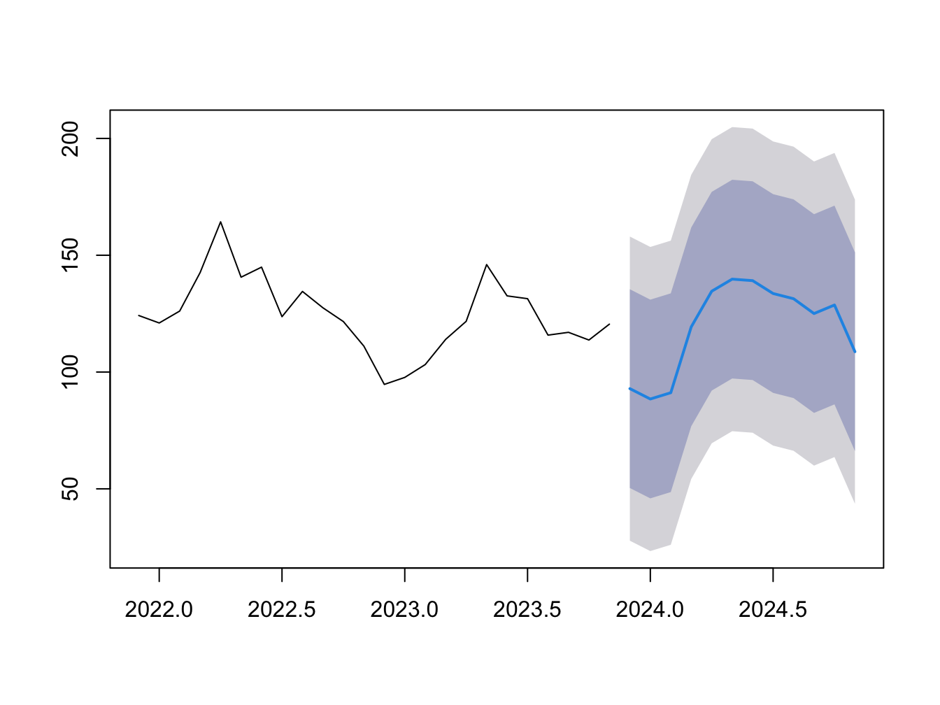
Figure 5.5: Forecast of Housing Starts