Chapter 4 Smoothing Methods
One way to approach forecasting is to average out the fluctuations in the underlying time series to produce a smoothed data which can be extrapolated to produce forecasts. These smoothing methods are essentially model-free and may not even produce optimal forecasts. Depending on the method used one can accommodate seasonal as well as trend components of the underlying time series.
4.1 Moving Average Method
We compute an average of most recent data values for the time series and use it as a forecast for the next period.
An important parameter is the window over which we take the average. Let us denote this window by \(m\), then: \[\begin{equation} y^s_{t+1}=\frac{\sum \limits_{i=t-m+1}^{t}{y_i}}{m} \end{equation}\]
A larger value of \(m\) produces greater smoothing and most software have a default value of this parameter which can be changed if needed.
4.2 Simple Exponential Smoothing
In the moving average method, all observations received same weight. However, it is reasonable to argue that more recent observations may have a greater influence than those in the remote past. In this method, the weight attached to past observations exponentially decay over time. Here is the algorithm for computing the smoothed data and its forecast:
Initialize at t=1: \[y_1^s=y_1\]
Update: \[y_{t}^{s}= \alpha y_t + (1-\alpha)y_{t-1}^{s} \quad for \ t=2,3,...T\]
3: h-period ahead forecast: \[f_{T,h}= y_T^s\]
Here the h-period ahead forecast is:
Exercise: Can you show that \(y_{t}^{s}\) is a is the weighted moving average of all past observations? Use backward substitution method.
Here \(\alpha \in (0,1)\) is the smoothing parameter, with smaller value indicating greater smoothing.
4.3 Holt-Winters Smoothing
We add trend component to the simple exponential smoothing. In step 2 the equation we use to update the smoothed data is given by:
\[\begin{align} y_{t}^{s}= \alpha y_t + (1-\alpha)(y_{t-1}^{s}+B_{t-1}) \\ \nonumber B_t = \beta (y_t^s -y_{t-1}^s) + (1-\beta) B_{t-1} \end{align}\]
We now have an additional parameter \(\beta\) that is the trend parameter. Here the h-period ahead forecast is:
\[\begin{align} f_{T,h} = y_T^s + h\times B_T \end{align}\]
4.4 Holt-Winters Smoothing with Seasonality
We now add seasonal component along with trend. Assuming multiplicative seasonality with period \(n\):
\[\begin{align} y_{t}^{s}= \alpha \frac{y_t}{S_{t-n}} + (1-\alpha)(y_{t-1}^{s}+B_{t-1})\\ B_t = \beta (y_t^s -y_{t-1}^s) + (1-\beta) B_{t-1}\\ S_t = \gamma\frac{y_t}{y_t^s}+(1-\gamma)S_{t-n} \end{align}\]
The h-period ahead forecast is given by:
\[\begin{equation} f_{T,h}= (y_T^s + h\times B_T) \times S_{T+h-n} \end{equation}\]
4.5 Application
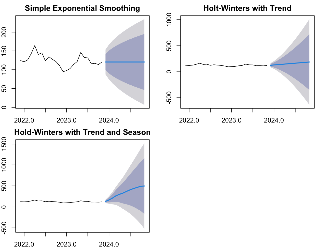
We use R to implement a 12-period ahead forecast for new housing starts for the U.S. The data is at monthly frequency from Jan 1959 through March 2019. The resulting forecasts are plotted in Figure 4.1.

Figure 4.1: Forecast of Housing Starts: Three Smoothing Methods